Plotting TTN gateways on a map

Introduction

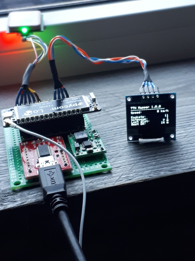
While using the TTN tracker application for some time now on my home-made LoPy tracker it shows that signals were recorded by at least 246 different gateways in the Dutch area. This raised a question: How many more did not yet receive my tracker, where are they located and which would be the easiest to drive by?
In my job as an IT consultant for Healthcare applications I drive all across The Netherlands so lots of opportunities to “take the long way home”.

The problem described has two parts: Gathering the gateways which received the tracker (A) and gathering the entire list of gateways (B). Plotting B minus A would be the answer.

Prequisits

This solution is built on NodeRed (0.19.4) with node-red-contrib-ttn (2.0.4) and node-red-contrib-web-worldmap (1.4.3) installed.

Which gateways received my tracker

I built this some time ago when the tracker was brought live and uses the TTN integration for Node-Red.SolutionA

Note: in contrib-ttn 2.0.4 the TTN message node is now called TTN uplink //post & picture needs update 🙂

The TTN message receiver is registered to the tracker application on The Things Network. On each received packet it sends an array of gateways (with tracker data, gateway ID, location, signal strengths etc) which received the particular packet. This data can be found in the msg.metadata part (not the ordinairy msg.payload). This array is decomposed and written to a CSV logfile. In the end this file contains all gateways, but not yet the unique list…

Contents of “Process received TTN messages:

//process new message which may contain the response
//of multiple gateways which received the packet
var gatewaysarray = msg.metadata.gateways;
var logMsgs = [];
for (i = 0; i < gatewaysarray.length; i++){
   logMsgs.push({payload: {time: gatewaysarray[i].time,
                           my_lat: lat_m,
                           my_lon: lon_m,
                           gtw_id: gatewaysarray[i].gtw_id,
                           channel: gatewaysarray[i].channel,
                           rssi: gatewaysarray[i].rssi,
                           snr: gatewaysarray[i].snr,
                           rf_chain: gatewaysarray[i].rf_chain,
                           gwy_lat: gatewaysarray[i].latitude,
                           gwy_lon: gatewaysarray[i].longitude,
                           dist: distancesarray[i],
                           }
                 });
   }
return logMsgs;

How to get the entire list of gateways

My first guess was asking JP Meijers of TTNMapper to build this list from his TTNMapper database. Although he was quite willing, a better suggestion was posed: This data is available through an API at TheThingsNetwork. The JSON reply looks like (shown for a single random gateway)

{“statuses”:
  {"eui-b827ebfffef23042":
    {"timestamp":"2018-04-21T10:44:03.020602294Z",
     "uplink":"52790",
     "downlink":"87",
     "location":
        {"latitude":50.06118,
         "longitude":9.459908,
         "altitude":260,
         "source":"REGISTRY"},
    "platform":"IMST + Rpi",
    "gps":
        {"latitude":50.06118,
        "longitude":9.459908,
        "altitude":260,
        "source":"REGISTRY"},
    "time":"1524307443020602294",
    "rx_ok":52790,
    "tx_in":87}

This JSON contains all we need to know.
One word of advice: This gateways JSON is about 5MB large. So we won’t do the TTN operators a favor when requesting these data every minute.

SolutioB

Upon receiving the (manual) trigger the second part of the flow first reads the entire CSV file with received packets created above and filters it to a single array of unique gateways which once received my tracker. The list is stored in the flow context for later use. Note: Of course if this application is the only purpose for this CSV logfile we could have done filtering right away i.e. only add to and save the unique list.

After retrieving the entire gateway list the results are filtered. I’m only interested in a rectangular area containing The Netherlands and gateways which have been online today.
From this data an array is formed containing the markers with for each marker the properties:

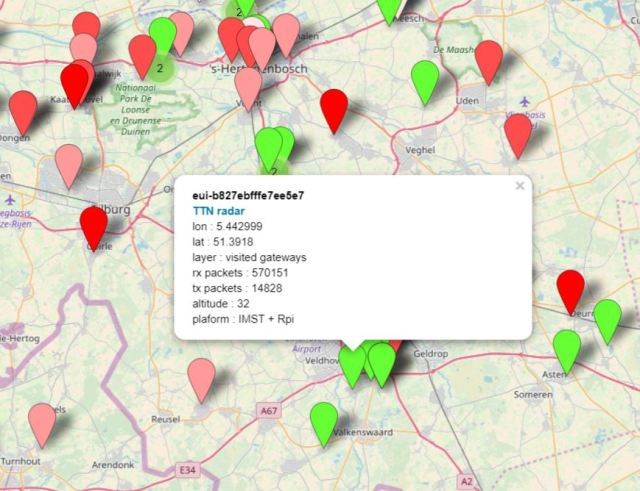
"name":key, // the gateway ID
"lon":gateways[key].location.longitude, //the gateway longitude
"lat":gateways[key].location.latitude, //the gateway lattitude
"layer": gwlayer, //the layer to put the marker on (either visited or new)
"icon": "dot-circle", //the icon used
"iconColor": gwcolor, //the color used: green or various reds depending on gwy activity
"weblink": weblink, //clickable url to TTNMapper radar for this gateway
"rx packets": gateways[key].uplink, //nr of received packets this gateway ever received
"tx packets": gateways[key].downlink, //nr of transmitted packets this gateway ever sent
"altitude": gateways[key].location.altitude, //gateway antenna height
"plaform": gateways[key].platform // type of hardware used.

Feeding this sequentially to the Node-Red Worldmap not only shows the gateways but lets us select the particular layer (seen or unseen gateways). Unseen gateways are colored according to their chance of being able to pick up the tracker. An indoor gateway with 100 packets received probably won’t hear the tracker at 2km distance.
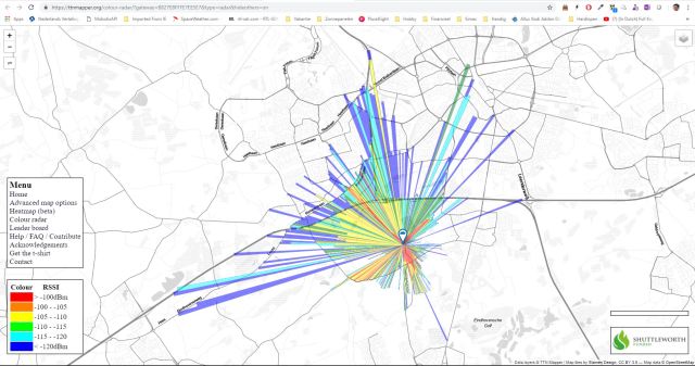
Clicking a gateway shows its details and a “TTN Radar link” to the TTNMapper radar page as well.

2018-09-21 10_41_44-Node-RED map all the things

2018-09-21 13_25_26-

Contents of Filter & Color:

var gwcolor = "";
var gwlayer = "";
var gwlist = [];

//only list gateways actively seen today
var d = new Date();
var todaystr = d.getFullYear() + "-" + ("0"+(d.getMonth()+1)).slice(-2) + "-" + ("0" + d.getDate()).slice(-2);
var gateways_seen = flow.get("gateways_seen");
var gateways = msg.payload.statuses;
node.status({fill:"red",shape:"dot",text:"Busy building list"});

//traverse through all existing gateways
//filter for The Netherlands area and active gateways only
//color seen gateways green, the others red intensity depending on nr of uplink messages
for (var key in gateways){
    if (gateways.hasOwnProperty(key)){
        if ((gateways[key].location.longitude > 2.8) &&
           (gateways[key].location.longitude < 7.6) &&            (gateways[key].location.latitude > 50) &&
           (gateways[key].location.latitude < 54) &&            (gateways[key].timestamp.substring(0,10) == todaystr)){                if (gateways_seen.indexOf(key) > -1 ){
                   gwcolor = "#66ff33";  //green
                   gwlayer = "visited gateways";
               }
                else {
                   gwlayer = "new gateways";
                   gwcolor = "#FFE6E6"; //very light red
                   if (gateways[key].uplink > 1000){
                      gwcolor = "#FF9999"; // bit brighter red
                      if (gateways[key].uplink > 10000){
                         gwcolor = "#FF4D4D"; // /another bit brighter red
                         if (gateways[key].uplink > 100000){
                            gwcolor = "#FF0000"; // absolutely red
                         }
                      }
                   }
                }
                //create URL to TTN Mapper radar page of this gateway
                //"eui-" type gateways need the eui part removed
                var newkey = key;
                if (key.substring(0, 4) == "eui-"){
                    newkey = key.substring(4).toUpperCase()
                }
                var weblink = {"name":"TTN radar", "url":"https://ttnmapper.org/colour-radar/?gateway=" + newkey + "&type=radar&hideothers=on"};
                //put marker in list to show
                gwlist.push({"name":key,  
                             "lon":gateways[key].location.longitude,
                             "lat":gateways[key].location.latitude,
                             "layer": gwlayer,
                             "icon": "", 
                             "iconColor": gwcolor, 
                             "weblink": weblink,
                             "rx packets": gateways[key].uplink,
                             "tx packets": gateways[key].downlink,
                             "altitude": gateways[key].location.altitude,
                             "plaform": gateways[key].platform
                });
           }
    }
}
node.status({});   // clear the status
flow.set("gwlist", gwlist);
msg = {payload: gwlist};
return msg;

Future developments

It would be great if the map would be realtime: As soon as the tracker is received by a gateway the marker could be updated realtime.

Download

A copy of the flows can be downloaded from my github pages

Enjoy!

Posted in The Things Network | Tagged , , , , | Leave a comment

Monitoring Linux based LoRa gateway

As a LoRa TTN gateway owner you want to know what’s going on at your gateway sooner or later. Now the gateway traffic page at The Things Network console offers some insights but it offers no API to get the info and graph it somehow, yet.

Owners of a Linux based gateway (like me) can monitor the IP traffic between the gateway and TheThingsNetwork servers which runs on port 1700. TTN Gateways however use MQTT to exchange data with TheThingsNetwork servers and this post does not apply.

At Hackaday  Bjorn Amann describes how tcpdump can be utilized to snoop the gateway traffic. Note that all LoRa traffic is encrypted so don’t expect to see real userdata, but we are interested in the metrics.

First we need to install tcpdump on the Gateway Raspberry Pi with

sudo apt-get install tcpdump

which should install the neccesary packages. Provided your gateway is connected by WLAN (like me) you could give it a testrun with.

sudo tcpdump port 1700 -s 500 -U -n -t -w - -i wlan0

If connected by Ethernet use eth0 instead of wlan0. The console should spit out data at least at 30 second intervals, but probably more. You might even recognize json parts starting with {“rxpk:”  These are the ones we’re interested in!

Some info on the parameters:

-s 500 = first 500 byte of packet
-U = don’t wait to fill buffer before sending
-n = no domain lookups
-t = give human readable timestamp output
-w – = write output
-i wlan0 = use wifi interface (change to eth0 on a wired gateway)

We will be using Node-Red to process the data and Domoticz to visualize it. Assume your Node-Red instance runs on a machine with IP address NodeRedIP and we will be using a random port “8888” to convey the data.

Now we start our snooping listerer in background and pipe the data to Node-Red with:

sudo tcpdump port 1700 -s 500 -U -n -t -w - -i wlan0 | nc NodeRedIP 8888 &

| = pipe output to
nc = netcat
NodeRedIP = ip to send data to
8888 = port to send data to
& = run in background

This will start sending data over a TCP pipe to Node-Red where we just need to receive it with a TCP node listening on port 8888. That’s it ! A succesful connection will show “1 connection” below the node.

Download the complete Node-Red project from my Github here.

Now the fun starts and the received data, available in the msg.payload as string, can be processed. In the Node-Red example the packets are first checked for rxpk (received packet) or txpk (transmit packet) or anything else (keepalive). Any packet will retrigger a watchdog timer which emails if no packet was received within 65 seconds meaning that the gateway went down.

Then the json is read from the data and the rest of it is discarded. We now have metadata for the received packet but not yet the node address (and thus the network it belongs to). We therefore need to decode de Base64 encoded data packet and get the additional info from there. This conversion requres you to install the node-red-node-base64 node using the nodes palette. All data together are formed into a single object for each received packet like this:

{“device”:113434400,”count”:437,”netid”:3,”tmst”:1573228548,”time”:”2018-04-22T15:45:25.034275Z”,”chan”:2,”rfch”:1,”freq”:868.5,”stat”:1,”modu”:”LORA”,”datr”:”SF10BW125″,”codr”:”4/5″,”lsnr”:-11.8,”rssi”:-117,”size”:54}

which we now can use to:

  1. store into a CSV file for later analysis (adapt file name/location)
  2. count the packets received
  3. count the unique devices seen on a day
  4. report the first of a number of packets from a TTN device (a tracker?)
  5. Watchdog your gateway (adapt email info in the email node)
  6. whatever comes to mind (keep a list of known trackers?)

Graphing is done in Domoticz using an incremental counter virtual device. Mark the IDX value in Domoticz and adjust the corresponding http request node in Node-Red. Eventually the graph in Domoticz will look somewhat like:

Enjoy!


Posted in Domoticz, LoRa, Node-Red | 4 Comments

LoRa 868 MHz collinear results

The antenna described in the previous post and the preliminary results encouraged me to get the thing on the roof. April 1st (no joke!) seemed the right time. Hardly any rain according to the radar. So i filled the bag with tools, tape and tywraps and… the gateway with the antenna. After some nerve-racking moves i found myself on the flat roof of our house. Then it started raining.

I could use the left over PVC pole of the ADSB antenna which moved to a higher spot two years ago. After some 20 minutes it was time for the photo shoot and safely move back in, all drenched. But excited to see if my gateway would be back online.

DSC0375_annoDSC03759_anno

360view

360 degrees panoramic view

DSC03754

Now, with the gear on the roof it’s time to drive around and check the new coverage. Thing look good, very good! But how to compare the current coverage with the previous?

Plotting with Basemap and Python

I decided to dive into the world of map plotting using Python. Mathplotlib and Basemap appear to be the defacto standard. So i installed both and managed to follow the guide from http://introtopython.org/visualization_earthquakes.html.  Then i downloaded the CSV data for my tracker node from TTNMapper.org for the past 2 weeks and filtered that data to my gateway. I downloaded a comparison dataset for the testdrive i just did and plotted RSSI radials for both datasets on the map. Compare the results:

Well worth the trouble i think! I did the same, now for the SNR values (ranging from -5 to +5 dB in steps of 2 dB). As expected the results are quite comparable.

Now let’s hope the Scotchfil will keep the rain from the cable…

20180402_143629

Posted in LoRa | Tagged , , , , , | 4 Comments

A LoRa 868MHz Collinear antenna

A warning ahead: the following is a YMMV project. Coax collinears have come in very different flavours and it is very hard to find at least two sources which agree on a reproducible design. Ok, they all consist of a number of halve wave segments corrected for the velocity factor of the coax used. But that’s about where the similarity ends.

Variations come in:

  • Top section
    • just end with a halve wave part,
    • left open,
    • shorted or even
    • ended with 50 ohm resistor
    • A quarter wave coax top section with a quater wave whip
  • Bottom section
    • Quarter wave coax section
    • Decoupling with
      • Radials
      • Sleeve
      • Ferrite core

Realizing this could well end in a frustration (i did some collinears for ADSB with mixed results) i started off with what i thought was a proper design. However, while building i didn’t put the bottom part together in the way it was planned.

While measuring the SWR with a N1201SA antenna tester it was impossible to tune the SWR by cutting the whip. Only after removing the complete quarterwave top end, the SWR got right. Tuned it a little more by cutting the top halve wave with a cm or so.

This is what the final design became:

CoaxCollinearLoRa


CoaxCollinearBottom

I used a N-connector pigtail cable (so the blue part is a little piece of RG174 coax).

Some pictures:


Having having done the tests and shooting the pictures the whole thing was glued together to prevent water from getting in.

Results and field tests

The most exciting part! As mentioned the SWR results were disappointing until the top quarterwave part was taken off (probably as a result of not building the bottom part as designed). When the antenna was properly tuned the SWR was stable even when moving or touching the coax feed: the radials do their job! Also detuning caused by the PVC tube was neglectable.

A temporarely gateway was setup to compare the field strength to two whip antenna’s (which tested to be nicely resonant at 868 MHz). A quick comparison showed the collinear to outperfom the whips. Promising!

20180326_230713

Reference Long and Short whip

Later that day i did some more tests at 530m from my gateway and 7.2km from the gateway at Eindhoven airport (FFFEB827EB75534E). My LoPy LoRa tracker was used as signal source. I used 3 types of antenna’s: Small whip, large whip and collinear. I left the tracker running for a few minutes to have a number of observations). At home the results were analyzed from the datafile Node-Red creates. RSSI values varied +/- 4 dB without touching anything. For each antenna the average of the RSSI values was calculated, resulting in:

Distance to gateway Eindhoven airport: 7.2 km

Short whip    avagage RSSI  -118 dBm   (11 packets)
Long whip    avagage RSSI   -115 dBm  (20 packets)
Collinear       avagage RSSI   -110 dBm  (14 packets)


Distance to home gateway: 530.

Short whip    avagage RSSI  -113 dBm   (13 packets)
Long whip    avagage RSSI   -108 dBm  (26 packets)
Collinear       avagage RSSI     -98 dBm  (16 packets)

Still promising and about what to be expected of this configuration! This weekend the gateway and the antenna will move to the rooftop. Results will be shared here!


Posted in LoRa | Tagged , , , | 11 Comments

Mapping The Things Network with a LoPy (4). Node-Red backend

This page will not go into the details on how to install and run Node-Red on a Raspberry Pi. Other resources about that can be found here and here.

A primer on how to use the TTN nodes in Node-Red can be found here

Messages from our Tracker node as received by any (some) of the TTN gateways are made available through the TTN Node-Red node. A received message not only contains the message itself but also the meta data which contains details on the gateways who recieved the me’ssage. Thus we can calculate the distance between LoRa sender and LoRa receiver(s).TTN mapper Node-RED

At the core is the function node which processes each received packet. It calculates the distance between receiver (from the array of gateways in the received meta data) and the sender (from the data in the actual message). It keeps track of the number of messages (packets) received and the number of unique gatways which received a message. The tracker itself will keep track of the longest distance of messages received so we don’t need to send that back to the tracker for display.

Apart from data being send back to the tracker the function also prepares data to be logged. By doing so we can later evaluate the results of our tracking journey. Also the  current location of the Tracker will be shown on the http://127.0.0.1:1880/worldmap page of Node-Red.

//function claculates distance between locations in meters
function getdistance(lat1, lon1, lat2, lon2) {
 var R = 6371000; // Radius of the earth in m
 var dLat = (lat2 - lat1) * Math.PI / 180;
 var dLon = (lon2 - lon1) * Math.PI / 180;
 var a = 
 0.5 - Math.cos(dLat)/2 + 
 Math.cos(lat1 * Math.PI / 180) * Math.cos(lat2 * Math.PI / 180) *
 (1 - Math.cos(dLon))/2;

return Math.ceil(R * 2 * Math.asin(Math.sqrt(a)));
}

//reset gateways, packets and couter if tracker did restart
var counter = flow.get("counter");
if (msg.counter < counter){
 gateways = 0;
 packets = 0;
 var unique_gateways = [];
} else {
 gateways = flow.get("gateways");
 packets = flow.get("packets");
 var unique_gateways = flow.get("unique_gateways"); 
}

flow.set("counter", msg.counter);

var lat_m = msg.payload_fields.latitude;
var lon_m = msg.payload_fields.longitude;

var gatewaysarray = msg.metadata.gateways;
var distancesarray = [];

//log received data on second port
var logMsgs = [];
var currentTime = new Date().getTime();

//process new packet
packets = packets + 1;
for (i = 0; i < gatewaysarray.length; i++){
 distancesarray[i] = getdistance(lat_m, lon_m, gatewaysarray[i].latitude, gatewaysarray[i].longitude);
 logMsgs.push({payload: {time: currentTime,
 my_lat: lat_m,
 my_lon: lon_m,
 gateway: gatewaysarray[i]
 }
 });
 if(unique_gateways.indexOf(gatewaysarray[i].gtw_id) == -1){
 //new gateway found
 unique_gateways.push(gatewaysarray[i].gtw_id);
 gateways = gateways + 1;
 }
}
var distance = Math.max(...distancesarray);


//store results of this packet
flow.set("gateways",gateways);
flow.set("unique_gateways", unique_gateways);
flow.set("packets",packets);

return [{
 dev_id: msg.dev_id,
 port: msg.port,
 payload: {
 packets: packets,
 gateways: gateways,
 distance: distance
 }
 },
 logMsgs
];


Note that data received from the tracking node and send back to it needs to be packed in a byte array to limit the number of bytes transferred over the wireless link. The conversion between a javascript object and the byte array is handled by the decoder and encoder found under “payload formats” of your application in The Things Network console.

The decoder will convert the packed payload as received from the Tracker by the gatewato a JS object while the encoder will encode the JS object Node-Red returns to reply it back to the Tracker which can then display it. Find the encoder and decoder as encoder.js and decoder.js on Github

Posted in LoRa | Tagged , , | 3 Comments

Mapping The Things Network with a LoPy (3). Wiring diagram

This part of the project will show the wiring diagram for the LoPy tracker.

Schematics

The tracker is built around the LoPy of PyCom. It’s a MicroPython programmable ESP32 with LoRa transceiver on board. Although one can connect to it using the device’s AP mode a serial to USB FT232R interface was used. This also powers the unit through the USB 5V. The LoPy has a 3.3V regulator on board capable of delivering 1.2A, well enough for the peripherals we will be adding.

Communication to the display uses I2C and the GPS module uses a UART port. During installation the FT232R was also used to connect and configure the GPS.

Most components were obtained through Banggood:

Some pictures for further inspiration

20180305_080409

20180306_215435

20180316_085610

In full operation

IMG-20180315-WA0004

Results as shown on TTN Mapper

Posted in LoRa | Tagged , , | 2 Comments

Mapping The Things Network with a LoPy (2). Programming the LoPy

The most interesting part is definitely the LoRa node for which i use a LoPy. The software described here is based on the work of PiAir found here on GitHub and taylored to my needs.

Before going into the software a few lessons learned regarding the use of the LoPy:

  • Memory constraints.

It is not possible to just load any python code and libraries. It won’t fit in the memory of the device. A solution for this is to load cross compiled python modules (aka “Frozen bytecode).  The only disadvantage is that debugging is more time consuming. A ready to use cross compiler is provided by @robert-hh on his github pages (look for mpy-cross_pycom.exe if you’re on Windows).

Another memory constraint is RAM. Performing a so called “Garbage collection” frees up memory and could avoid hard to track errors. In my case i used to get a timeout error on sending a LoRa packet after some 50 packets (which are still being catched just in case). This behaviour was not seen again after doing a gc.collect() call every sending loop.

  • Take care not to assign pins twice

This may sound a no brainer but when using 4 ports (UART0 for terminal, LoRa module on SPI at pin p5, p6 and p7), I2C for the display on p8, p9 and UART1 for the GPS on pin p11, p12) an error is easily made.

  • Do not search for internet in STA mode

Normally one would try to login to the home WiFi in the boot.py module. This is nice when developing but out in the car/on the bike there is little chance that the WiFi could be found which would stall the boot process.

  • Uploading using ampy (adafruit)

How to upload code then? Having played around with Atom and its Pymakr plugin i got an “unable to upload” too often so a reliable serial uploader was searched. Adafruit provides “ampy“, a commandline uploader which never failed (provided you close any open Putty sessions to the same port). Ampy provides basic commands like “ls”, “put” etc and is invoked like: C:>ampy –port COM4 put main.py

  • Prefer ABP over OTAA ?

Actually this still hasn’t been decided on. While driving around it might take a while for the tracker to be able to join the LoRaWAN network. Leaving from home this is no problem as i run my own gateway, but anywhere else this could take longer than the patience permits. ABP should have the node joined right away (did not try this mode yet) but requires storing the message counter. Anyway, follow the latest here

  • Use cold Reboot (soft restart will not restart the LoRa module)

Soft booting the LoPy (Ctrl-D in REPL terminal) will have you waiting for a LoRaWAN join forever. The thing just won’t transmit any packet at all. A cold restart will, but in my experience it may take a try or two to have it start the boot.py (probably due to this). Will ask around how to have this more predictable. Follow progress here.

The software can be found on my github pages. Instead of uploading the .py versions grab the .mpy files from the obj directory to save memory. Note that if both the .py and .mpy files are found it will still try to compile and waste memory.

Before uploading change the config.py to your needs. (optional) WiFi settings, ports used and most important: the  APP_EUI  and APP_KEY as found in your The Things Network console when drilling down to the particular device you’ve registered.

Usage

Following steps will be performed after reboot:

  1. Led falshes RED while waiting for WiFi (if configured)
  2. Display initializes at all “0”
  3. Led flashes YELLOW while waiting for OTAA registration on the LoRa network. Depending on nearby gateway availability this may take a while
  4. Led flashes BLUE while waiting for GPS fix. Depending on the skyview this might take a while.
  5. Led flashes GREEN. Yes! You’re there. The location will be sent roughly every 10 seconds. While sending and waiting for a reply from the network the led will be PURPLE
  6. Received data will be shown on the display and the time should show the actual UTC time. During LoRa transmit/receive the time will stop for a few seconds.


Posted in LoRa | Tagged , , , , | Leave a comment

Mapping The Things Network with a LoPy (1) Introduction

Welcome to my pages. If you landed here there must be at least some interest in either The Things Network, mapping its coverage or the LoPy, Pycom’s LoRa enabled controller. If neither is the case you’re still invited to read on and have yourself carried away into the world of Internet of Things…

As a proud owner of a WiPy, Pycom’s first WiFi enabled MicroPython programmable micro controller and of which i briefly blogged a while ago, i could not resist to buy its ESP32 based successor: The LoPy. The LoPy even ads the LoRa protocol and Bluetooth. The device collected quite some dust until i got to know The Things Network: An open Internet of Things wide area network using LoRa technology.

Soon i owned a gateway  (based on a RAK831 and RPi Zero) and was curious what its range would be. This is where TTN Mapper comes in. The idea is simple: Driving around with a LoRa transmitter which sends out a message say, each 15 seconds, your signal might be picked up by one or more gateways. An Android App registered to The Things Network waits for messages being reported. Knowing your location (GPS enabled on the SmartPhone) the App can now report the distance(s) and RSSI value(s) for this particular location and the particular gateway(s).  The principle is shown by it’s developer JP Meijers in a video.

Another possibility is to have the mobile node send it’s GPS location on regular intervals enabling TTN Mapper to process the data without the need of a SmartPhone. This however does not provide the driver with the feedback (and joy!) that his 25mW 868Mhz signal has been picked up by a sometimes 10 km remote gateway. Using this together with the App is no problem. TTN Mapper will be happy if a packet is accompanied by two locations (one from the packet itself and one from the App). Still it would be great if there was some other way of getting feedback.

So… why not use LoRa for this?

Sparked by this discussion (many thanks to  user piair for starting it) i decided to give this idea a try. The result should be that the number of gateways, distance, largest distance and received packets is displayed on the tracker device without the need of a SmartPhone. It will look like this:

TTNMapper

The end result should look like this

In short: The LoPy receives it’s locations (LON1, LAT1) from a GPS module over a serial connection. This location is encoded and transmitted over LoRa. When a gateway receives this packet it is forwarded to TTN Mapper. It will also be decoded and send to my Node-Red application at home. As this data also contains the metadata (with the locations of all gateways which received the packet) the largest distance can now be derived. The number of received packets is incremented, the number of unique gateways counted and replied back to the node over LoRaWAN (encoded in a 5 byte string). This data will be scheduled and fed back to the LoPy following the next received uplink packet. The LoPy on its turn can now display these statistics and as a bonus keep track of the current speed and largest LoRa distance as well.

In the next post i will further dive into the specifics of the code and configurations involved and the hurdles taken to get things running.

Posted in LoRa | Tagged , , , | 4 Comments

Using Node-Red to graph scale data

Having used Node-Red briefly about two years ago, i decided to load it again onto the Raspberry Pi which listens for my BS440 scale. Just to dig into Node-Red and see where it got.

Installing Node-Red is a breeze although it takes a coffee and a beer or two before it is installed. But it’s more than worth the wait! A newly added set of nodes is the “dashboard” which can be added through the palette manager once Node-Red is up and running.

My idea was that i could graph the BS440 scale data which is stored into a CSV file (if the CSV plugin is enabled). I was shocked to find out i had made a fully operational webpage showing the data within one hour of coding (or drawing to be more precise)! And that included getting  familiar with Node-Red.

The result is a fancy looking page which shows nicely on my SmartPhone and is lightning fast. It offers a drop down selection for the type of data and two buttons to select the user. Ain’t that cool!

So how is this done? Without giving a lecture on Node-Red (i’ll leave it up to you to explore this piece of magic) this is what the flow looks like:

NR-BS440-flow

The core is reading the CSV file. The filename is set by selecting a user and is called 1.csv for user 1, 2.csv for user 2 etc. The CSV BS440 gives me uses a plain comma to separate its values and has no header like the data below:

1586929481,76.2,14.0,36.7,2.9,68.0,3254,23.0
1587019687,75.5,13.8,36.8,2.9,68.2,3236,22.8
1587102926,76.3,14.0,36.7,2.9,68.0,3257,23.0
1587356357,77.0,14.3,36.6,2.9,67.8,3275,23.2
1587356428,77.3,14.5,36.5,2.9,67.7,3283,23.3
1587416013,77.2,14.4,36.5,2.9,67.7,3280,23.3
1587416075,77.2,14.4,36.5,2.9,67.7,3280,23.3
1587416234,77.3,14.4,36.5,2.9,67.7,3283,23.3
1587447935,76.5,14.1,36.6,2.9,67.9,3262,23.1
1587533240,76.1,14.0,36.7,2.9,68.0,3252,23.0
1587621367,75.5,13.7,36.9,2.9,68.2,3236,22.8
1587706556,75.7,13.9,36.8,2.9,68.1,3241,22.9

Hence we need to convert the data to a JS object and assume columns as

time, weight, fat, muscels, bones, moisture, calories,BMI

CSV

Once the file is read it is converted to a node-js object. Type selects which data we want to graph. The selected type of data is read from the object and fed into the graph node.

The selecting thing might need some explanation as it uses JSONata (just watch the video). It is included in Node-Red and enables you to make a query from a bunch of JSON formatted data in just a single statement. As an example. If you want to craft an array of “vet” values from all data and change the unix timestamp to show milliseconds on the fly the JSONata for that is just:

[ { “key”: “vet”, “values”: msg.payload.[tijd*1000, vet] } ]

and the node “Select vet”  then looks like (note the J: selection)

NR-BS440-4

The rest of the nodes just show the dropdown list and store and show the current user.

The project is made available on my Github

On to the next project. Lets have fun!

Posted in BLE | Tagged , , , , , , , | 10 Comments

Connecting the Medisana BS440 Bluetooth scale (epilogue)

Having used the BS440 bathroom scale script for over a year i got time to update the whole thing. I decided to do a full reinstall and log all the individual steps it takes to get things running. So here is the recipe.

Hardware:

  • Raspberry Pi B+ (note: i have no Pi3 so no experience in using the built in BLE adapter)
  • USB BLE adapter (I use brand ADJ model 100-00006 BT 4.0 adapter which uses driver broadcom BCM20702A0)
  • WiFI adapter (unless you can position a wired RPi within 1 m from the scale) like this one
  1. Download latest Raspbian Jessie Lite build for your RPi from here.
  2. Format and image the SD card. Instructions here
  3. Enable SSH access by placing a file named ‘ssh’, without any extension, onto the boot partition of the SD card.
  4. Use a temporarely wired connection to connect to the RPi using Putty
  5. Change pwd and run sudo raspi-config and do
    expand filesystem
    set timezone
    set hostname like bs440rpi (or any other nice name)
  6. run sudo apt-get update and sudo apt-get dist-upgrade
  7. Enable WiFi using this tutorial.
  8. Follow Tony DiCola tutorial to set up Bluez on the RPi. I selected the latest and greatest Bluez 5.44. Follow this tutorial step by step. No need to enable “experimental”. Building Bluez will take half an hour or so…
  9. Copy btmgmt to the local bin folder with:  sudo cp /home/pi/bluez-5.44/tools/btmgmt  /usr/local/bin so it can be used from anywhere.
  10. Enable BT low enegry with btmgmt le on
  11. run hcitool lescan  and step on the scale with a registered user selected so all your properties are measured and stored. The scale should report with its MAC address and name like F1:37:57:6C:DE:64 [0202B664DE6C5737F1] write down both.
  12. Test connectivity with sudo gatttool -t random -b F1:37:57:6C:DE:64 -I
  13. at the prompt type connect which should respond connected. Error 111 indicates that the adapter is not in LE mode (retry the btmgmt le on).
  14. Avoid having to use super user privileges (sudo) on hcitool by sudo setcap 'cap_net_raw,cap_net_admin+eip' `which hcitool`
  15. Avoid having to use super user privileges (sudo) on btmgmt by sudo setcap 'cap_net_raw,cap_net_admin+eip' `which btmgmt`
  16. Install Pygatt 3.0.0 by sudo apt-get install python-pip and sudo pip install "pygatt[GATTTOOL]" This will throw a number of warnings and even errors but should end with Successfully installed pygatt pyserial enum34 pexpect ptyprocess
  17. Get the BS440 files by downloading the zip file from https://github.com/keptenkurk/BS440  and put them in a separate folder on the RPi like /home/pi/BS440.
  18. Enable the plugins of your choice by removing the underscore in the plugins folder for the .py and .ini files.
  19. Edit BS440.ini (fill in your scale’s MAC address and name from step 11) and all the enabled BS440<plugin>.ini in the plugins folder
  20. Start BS440.py with  python BS440.py. Start a second shell and monitor the logfile with tail -f BS440.log
  21. Enjoy
Posted in BLE | 14 Comments